Strathclyde's Changing Demographics
How gender balance, capacity and student origin shifted at the University of Strathclyde between 2014/15 and 2022/23.
I am a big fan of journalism — The Economist in particular — so I thought it would be fun to try a bit of data journalism of my own and pitch it to my university newspaper. I started by looking into the demographics of the University of Strathclyde; what follows is a short report on what changed.
Over the years Strathclyde has been through a lot: Brexit, Covid and strikes may all have left a mark on the university’s make-up and capacity. This report goes to the data to see which trends actually show up.
Gender
Of Boys and Men: Why the Modern Male Is Struggling, Why It Matters, and What to Do About It, published in 2022 by the British author Richard Reeves, argues that the modern male is being left behind in education. This correspondent read it — and the same pattern appears at Strathclyde, which has become more female-dominated with no sign of the trend slowing.
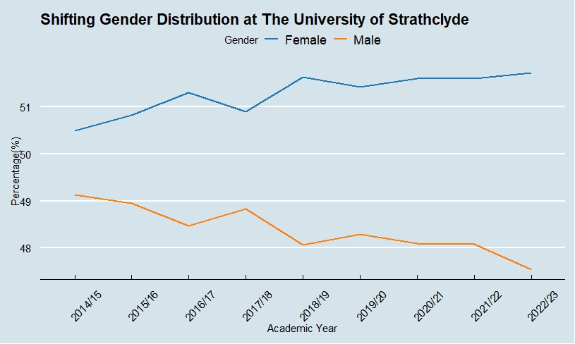
The gender gap has doubled: from roughly 51% female to 49% male, to around 53% female and 47% male. Filter the data to full-time students, though, and a different picture emerges — close to the 50:50 split one would expect.
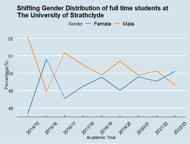
The explanation is that most part-time students are female. Why that is can only be speculated on, but on full-time numbers Strathclyde is a well-balanced university, which is attractive to a lot of applicants.
Permanent Address
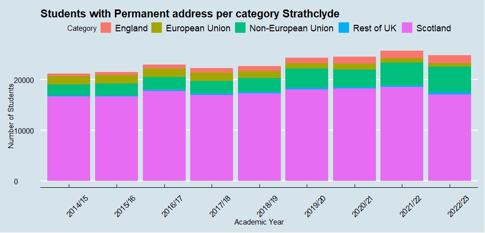
Strathclyde’s capacity has expanded from 21,210 students in 2014/15 to 24,860 in 2022/23, the most recent year this correspondent could get data for. That is an increase of more than 17% in eight years, reflecting the rising demand for higher education. What the headline number doesn’t show is where those extra students come from.
Looking at non-Scottish students, there is a clear rise in students from outside Scotland. This trend is significant to the University as Scottish students get the first degree for free or pay £1,920 per year, compared to the rest of the UK that pays £9,250 per year, with international fees ranging from £19,850-£29,350 for the academic year of 2025/26
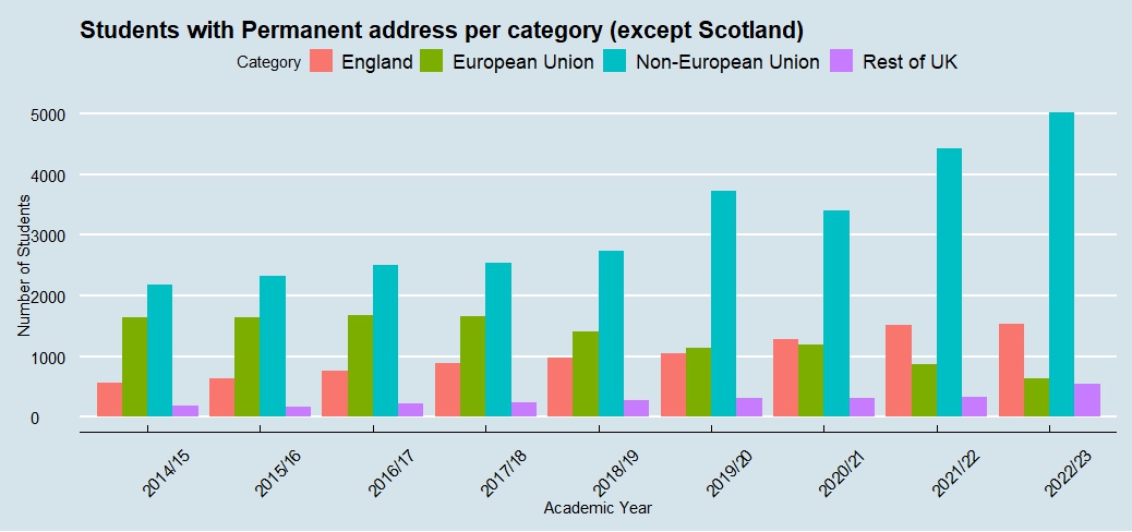
Across the eight years the campus has taken in steadily more students whose permanent address is abroad. The one exception to the trend is the EU, most likely a consequence of Brexit. The international student population has doubled in eight staggering years. That lets the university charge higher fees to cover its costs — but the same economic incentive leaves less room for Scottish students, who pay the least and bring the university the least money.
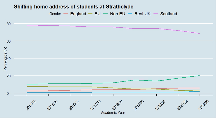
Scottish students are on the decline, while non-EU students make up over 20% of the population in 2022/23, up from around 10% in 2014/15. Scottish students now account for roughly 70%, an absolute decrease of 10 percentage points since 2014/15. More diversity and the extra resources that come with international students should be welcome, but the cost may be less space for Scottish students: their number in 2022/23 is the lowest since 2014/15, even though the university added places overall.
Data source: HESA — students data and analysis
The code is below. There are plenty of ways it could be more efficient; if I rewrote it today I would factor the repeated data-loading into a single function.
#Strath students demographic

#Library
library(readr) # reading csv
library(dplyr) #select package
library(ggplot2)
library(tidyr)
library(ggthemes)
setwd("C:\\Users\\example")# change this to the address of the data

#Sorting out the data
{
#2022-2023
{
strath_2022_2023 <- read_csv("table-1-(2022-23).csv", skip=14)
strath_2022_2023_filtered <- strath_2022_2023 %>%
  filter(`HE provider` == "The University of Strathclyde")
students2022_2023 <-  strath_2022_2023_filtered %>%
  filter(`Country of HE provider` == "All") %>%
  filter(`Region of HE provider` == "All") %>%
  filter(`Entrant marker` == "All") %>%
  filter(`Level of study` == "All") %>%
  filter(`Mode of study` == "All")

students2022_2023 <- students2022_2023 %>% select(-(c(`Country of HE provider`,`Region of HE provider`,`Entrant marker`,`Level of study`,`Mode of study`)))
}
#2021-2022
{
  strath_2021_2022 <- read_csv("table-1-(2021-22).csv", skip=14)
  strath_2021_2022_filtered <- strath_2021_2022 %>%
    filter(`HE provider` == "The University of Strathclyde")
  students2021_2022 <-  strath_2021_2022_filtered %>%
    filter(`Country of HE provider` == "All") %>%
    filter(`Region of HE provider` == "All") %>%
    filter(`Entrant marker` == "All") %>%
    filter(`Level of study` == "All") %>%
    filter(`Mode of study` == "All")

  students2021_2022 <- students2021_2022 %>% select(-(c(`Country of HE provider`,`Region of HE provider`,`Entrant marker`,`Level of study`,`Mode of study`)))
}
#2020-2021
{
  strath_2020_2021 <- read_csv("table-1-(2020-21).csv", skip=14)
  strath_2020_2021_filtered <- strath_2020_2021 %>%
    filter(`HE provider` == "The University of Strathclyde")
  students2020_2021 <-  strath_2020_2021_filtered %>%
    filter(`Country of HE provider` == "All") %>%
    filter(`Region of HE provider` == "All") %>%
    filter(`Entrant marker` == "All") %>%
    filter(`Level of study` == "All") %>%
    filter(`Mode of study` == "All")

  students2020_2021 <- students2020_2021 %>% select(-(c(`Country of HE provider`,`Region of HE provider`,`Entrant marker`,`Level of study`,`Mode of study`)))
}
#2019-2020
{
  strath_2019_2020 <- read_csv("table-1-(2019-20).csv", skip=14)
  strath_2019_2020_filtered <- strath_2019_2020 %>%
    filter(`HE provider` == "The University of Strathclyde")
  students2019_2020 <-  strath_2019_2020_filtered %>%
    filter(`Country of HE provider` == "All") %>%
    filter(`Region of HE provider` == "All") %>%
    filter(`Entrant marker` == "All") %>%
    filter(`Level of study` == "All") %>%
    filter(`Mode of study` == "All")

  students2019_2020 <- students2019_2020 %>% select(-(c(`Country of HE provider`,`Region of HE provider`,`Entrant marker`,`Level of study`,`Mode of study`)))
}
#2018-2019
{
  strath_2018_2019 <- read_csv("table-1-(2018-19).csv", skip=14)
  strath_2018_2019_filtered <- strath_2018_2019 %>%
    filter(`HE provider` == "The University of Strathclyde")
  students2018_2019 <-  strath_2018_2019_filtered %>%
    filter(`Country of HE provider` == "All") %>%
    filter(`Region of HE provider` == "All") %>%
    filter(`Entrant marker` == "All") %>%
    filter(`Level of study` == "All") %>%
    filter(`Mode of study` == "All")

  students2018_2019 <- students2018_2019 %>% select(-(c(`Country of HE provider`,`Region of HE provider`,`Entrant marker`,`Level of study`,`Mode of study`)))
}
#2017-2018
{
  strath_2017_2018 <- read_csv("table-1-(2017-18).csv", skip=14)
  strath_2017_2018_filtered <- strath_2017_2018 %>%
    filter(`HE provider` == "The University of Strathclyde")
  students2017_2018 <-  strath_2017_2018_filtered %>%
    filter(`Country of HE provider` == "All") %>%
    filter(`Region of HE provider` == "All") %>%
    filter(`Entrant marker` == "All") %>%
    filter(`Level of study` == "All") %>%
    filter(`Mode of study` == "All")

  students2017_2018 <- students2017_2018 %>% select(-(c(`Country of HE provider`,`Region of HE provider`,`Entrant marker`,`Level of study`,`Mode of study`)))
}
#2016-2017
{
  strath_2016_2017 <- read_csv("table-1-(2016-17).csv", skip=14)
  strath_2016_2017_filtered <- strath_2016_2017 %>%
    filter(`HE provider` == "The University of Strathclyde")
  students2016_2017 <-  strath_2016_2017_filtered %>%
    filter(`Country of HE provider` == "All") %>%
    filter(`Region of HE provider` == "All") %>%
    filter(`Entrant marker` == "All") %>%
    filter(`Level of study` == "All") %>%
    filter(`Mode of study` == "All")

  students2016_2017 <- students2016_2017 %>% select(-(c(`Country of HE provider`,`Region of HE provider`,`Entrant marker`,`Level of study`,`Mode of study`)))
}
#2015-2016
{
  strath_2015_2016 <- read_csv("table-1-(2015-16).csv", skip=14)
  strath_2015_2016_filtered <- strath_2015_2016 %>%
    filter(`HE provider` == "The University of Strathclyde")
  students2015_2016 <-  strath_2015_2016_filtered %>%
    filter(`Country of HE provider` == "All") %>%
    filter(`Region of HE provider` == "All") %>%
    filter(`Entrant marker` == "All") %>%
    filter(`Level of study` == "All") %>%
    filter(`Mode of study` == "All")

  students2015_2016 <- students2015_2016 %>% select(-(c(`Country of HE provider`,`Region of HE provider`,`Entrant marker`,`Level of study`,`Mode of study`)))
}
#2014-2015
{
  strath_2014_2015 <- read_csv("table-1-(2014-15).csv", skip=14)
  strath_2014_2015_filtered <- strath_2014_2015 %>%
    filter(`HE provider` == "The University of Strathclyde")
  students2014_2015 <-  strath_2014_2015_filtered %>%
    filter(`Country of HE provider` == "All") %>%
    filter(`Region of HE provider` == "All") %>%
    filter(`Entrant marker` == "All") %>%
    filter(`Level of study` == "All") %>%
    filter(`Mode of study` == "All")

  students2014_2015 <- students2014_2015 %>% select(-(c(`Country of HE provider`,`Region of HE provider`,`Entrant marker`,`Level of study`,`Mode of study`)))
}

#main is the origin of all merged df
{
main_dt <- full_join(students2022_2023, students2021_2022)
main_dt <- full_join(main_dt, students2020_2021)
main_dt <- full_join(main_dt, students2019_2020)
main_dt <- full_join(main_dt, students2018_2019)
main_dt <- full_join(main_dt, students2017_2018)
main_dt <- full_join(main_dt, students2016_2017)
main_dt <- full_join(main_dt, students2015_2016)
main_dt <- full_join(main_dt, students2014_2015)
}
}
# Gender related all students
{
gender_data <- main_dt %>%
  filter(`Category marker` == "Sex") %>%
  #filter(`Mode of study` == "All") %>%
  select(`Academic Year`, Category, Number) %>%
  spread(key = Category, value = Number)

# Calculate percentages
gender_data <- gender_data %>%
  mutate(Total = Female + Male + Unknown,
         Female_Percent = (Female / Total) * 100,
         Male_Percent = (Male / Total) * 100,
         Unknown_Percent = (Unknown / Total) * 100)


#gender_data <- sort_by.data.frame(gender_data, gender_data$`Academic Year`, decreasing = TRUE)
# Gender distribution over time
ggplot(gender_data, aes(x = `Academic Year`, group = 1), size = 1) +
  geom_line(aes(y = Female_Percent, color = "Female"),size = 1) +
  geom_line(aes(y = Male_Percent, color = "Male"),size = 1) +
  #geom_line(aes(y = Unknown_Percent,x = `Academic Year`, color = "Unknown"), size = 1) +
  scale_color_manual(values = c("Female" = "#1f77b4", "Male" = "#ff7f0e", "Unknown" = "#2ca02c")) +
  labs(title = "Shifting Gender Distribution at The University of Strathclyde",
       x = "Academic Year", y = "Percentage(%)",
       color = "Gender") +
  theme_economist() +
  theme(axis.text.x = element_text(angle = 45, hjust = 0))
}
#Residence stuff
{

#cleaning and grouping the data

  df_clean <- residence_data %>%
    filter(!Category %in% c("Total", "Total Non-UK", "Total UK"))

  df_with_sum <- df_clean %>%
    # Filter rows for 'Other UK', 'Wales', and 'Northern Ireland'
    filter(Category %in% c("Other UK", "Wales", "Northern Ireland")) %>%
    # Group by academic year and sum these categories
    group_by(`Academic Year`) %>%
    summarise(Number = sum(Number)) %>%
    mutate(Category = "Rest of UK") %>%
    ungroup()


  df_final_percent <- bind_rows(df_clean, df_with_sum) %>%
    # Filter out specific categories as needed
    filter(!Category %in% c("Other UK", "Wales", "Northern Ireland", "Not known")) %>%
    # Calculate the total number of students per year
    group_by(`Academic Year`) %>%
    mutate(Total_Year = sum(Number)) %>%
    # Calculate the percentage of each category for the year
    mutate(Percentage = (Number / Total_Year) * 100) %>%
    ungroup()

  # Combine the two dataframes together
  df_final <- bind_rows(df_clean, df_with_sum)  %>%
    filter(!Category %in% c("Other UK", "Wales", "Northern Ireland", "Not known", "Scotland"))


  ggplot(df_final_percent, aes(x = `Academic Year`, y = Number, fill = Category)) +
    geom_bar(stat = "identity") +
    labs(
      title = "Students with Permanent address per category Strathclyde",
      x = "Academic Year",
      y = "Number of Students",
      fill = "Category"
    ) +
    theme_economist() +
    theme(axis.text.x = element_text(angle = 45, hjust = 0))

  ggplot(df_final, aes(x = `Academic Year`, y = Number, fill = Category)) +
    geom_bar(stat = "identity",position = "dodge") +
    labs(
      title = "Non-Scottish permemant address for Strathclyde",
      x = "Academic Year",
      y = "Number of Students",
      fill = "Category"
    ) +
  theme_economist() +
    theme(axis.text.x = element_text(angle = 45, hjust = 0))


  #looking at perdentage changes

  category_percentage <- df_final_percent %>%

    select(`Academic Year`, Category, Number) %>%
    spread(key = Category, value = Number)

  # Calculate percentages
  category_percentage <- category_percentage %>%
    mutate(Total = England + `European Union` + `Non-European Union`+ `Rest of UK` + Scotland,
           England_Percent = (England / Total) * 100,
           EU_Percent = (`European Union` / Total) * 100,
           Non_EU_Percent = (`Non-European Union` / Total) * 100,
           Rest_UK_Percent = (`Rest of UK` / Total) * 100,
           Scotland_Percent = (Scotland / Total) * 100)

  ggplot(category_percentage, aes(x = `Academic Year`, group = 1), size = 1) +
    geom_line(aes(y = England_Percent, color = "England"),size = 1) +
    geom_line(aes(y = EU_Percent, color = "EU"),size = 1) +
    geom_line(aes(y = Non_EU_Percent, color = "Non EU"),size = 1) +
    geom_line(aes(y = Rest_UK_Percent, color = "Rest UK"),size = 1) +
    geom_line(aes(y = Scotland_Percent, color = "Scotland"),size = 1) +
    #geom_line(aes(y = Unknown_Percent,x = `Academic Year`, color = "Unknown"), size = 1) +
    #scale_color_manual(values = c("Female" = "#1f77b4", "Male" = "#ff7f0e", "Unknown" = "#2ca02c")) +
    labs(title = "Shifting home address of students at Strathclyde",
         x = "Academic Year", y = "Percentage(%)",
         color = "Gender") +
    theme_economist() +
    theme(axis.text.x = element_text(angle = 45, hjust = 0))
}


#Sorting out the data this time to do full time students
{
  #2022-2023
  {
    strath_2022_2023 <- read_csv("table-1-(2022-23).csv", skip=14)
    strath_2022_2023_filtered <- strath_2022_2023 %>%
      filter(`HE provider` == "The University of Strathclyde")
    students2022_2023 <-  strath_2022_2023_filtered %>%
      filter(`Country of HE provider` == "All") %>%
      filter(`Region of HE provider` == "All") %>%
      filter(`Entrant marker` == "All") %>%
      filter(`Level of study` == "All") %>%
      filter(`Mode of study` == "Full-time")

    students2022_2023 <- students2022_2023 %>% select(-(c(`Country of HE provider`,`Region of HE provider`,`Entrant marker`,`Level of study`,`Mode of study`)))
  }
  #2021-2022
  {
    strath_2021_2022 <- read_csv("table-1-(2021-22).csv", skip=14)
    strath_2021_2022_filtered <- strath_2021_2022 %>%
      filter(`HE provider` == "The University of Strathclyde")
    students2021_2022 <-  strath_2021_2022_filtered %>%
      filter(`Country of HE provider` == "All") %>%
      filter(`Region of HE provider` == "All") %>%
      filter(`Entrant marker` == "All") %>%
      filter(`Level of study` == "All") %>%
      filter(`Mode of study` == "Full-time")

    students2021_2022 <- students2021_2022 %>% select(-(c(`Country of HE provider`,`Region of HE provider`,`Entrant marker`,`Level of study`,`Mode of study`)))
  }
  #2020-2021
  {
    strath_2020_2021 <- read_csv("table-1-(2020-21).csv", skip=14)
    strath_2020_2021_filtered <- strath_2020_2021 %>%
      filter(`HE provider` == "The University of Strathclyde")
    students2020_2021 <-  strath_2020_2021_filtered %>%
      filter(`Country of HE provider` == "All") %>%
      filter(`Region of HE provider` == "All") %>%
      filter(`Entrant marker` == "All") %>%
      filter(`Level of study` == "All") %>%
      filter(`Mode of study` == "Full-time")

    students2020_2021 <- students2020_2021 %>% select(-(c(`Country of HE provider`,`Region of HE provider`,`Entrant marker`,`Level of study`,`Mode of study`)))
  }
  #2019-2020
  {
    strath_2019_2020 <- read_csv("table-1-(2019-20).csv", skip=14)
    strath_2019_2020_filtered <- strath_2019_2020 %>%
      filter(`HE provider` == "The University of Strathclyde")
    students2019_2020 <-  strath_2019_2020_filtered %>%
      filter(`Country of HE provider` == "All") %>%
      filter(`Region of HE provider` == "All") %>%
      filter(`Entrant marker` == "All") %>%
      filter(`Level of study` == "All") %>%
      filter(`Mode of study` == "Full-time")

    students2019_2020 <- students2019_2020 %>% select(-(c(`Country of HE provider`,`Region of HE provider`,`Entrant marker`,`Level of study`,`Mode of study`)))
  }
  #2018-2019
  {
    strath_2018_2019 <- read_csv("table-1-(2018-19).csv", skip=14)
    strath_2018_2019_filtered <- strath_2018_2019 %>%
      filter(`HE provider` == "The University of Strathclyde")
    students2018_2019 <-  strath_2018_2019_filtered %>%
      filter(`Country of HE provider` == "All") %>%
      filter(`Region of HE provider` == "All") %>%
      filter(`Entrant marker` == "All") %>%
      filter(`Level of study` == "All") %>%
      filter(`Mode of study` == "Full-time")

    students2018_2019 <- students2018_2019 %>% select(-(c(`Country of HE provider`,`Region of HE provider`,`Entrant marker`,`Level of study`,`Mode of study`)))
  }
  #2017-2018
  {
    strath_2017_2018 <- read_csv("table-1-(2017-18).csv", skip=14)
    strath_2017_2018_filtered <- strath_2017_2018 %>%
      filter(`HE provider` == "The University of Strathclyde")
    students2017_2018 <-  strath_2017_2018_filtered %>%
      filter(`Country of HE provider` == "All") %>%
      filter(`Region of HE provider` == "All") %>%
      filter(`Entrant marker` == "All") %>%
      filter(`Level of study` == "All") %>%
      filter(`Mode of study` == "Full-time")

    students2017_2018 <- students2017_2018 %>% select(-(c(`Country of HE provider`,`Region of HE provider`,`Entrant marker`,`Level of study`,`Mode of study`)))
  }
  #2016-2017
  {
    strath_2016_2017 <- read_csv("table-1-(2016-17).csv", skip=14)
    strath_2016_2017_filtered <- strath_2016_2017 %>%
      filter(`HE provider` == "The University of Strathclyde")
    students2016_2017 <-  strath_2016_2017_filtered %>%
      filter(`Country of HE provider` == "All") %>%
      filter(`Region of HE provider` == "All") %>%
      filter(`Entrant marker` == "All") %>%
      filter(`Level of study` == "All") %>%
      filter(`Mode of study` == "Full-time")

    students2016_2017 <- students2016_2017 %>% select(-(c(`Country of HE provider`,`Region of HE provider`,`Entrant marker`,`Level of study`,`Mode of study`)))
  }
  #2015-2016
  {
    strath_2015_2016 <- read_csv("table-1-(2015-16).csv", skip=14)
    strath_2015_2016_filtered <- strath_2015_2016 %>%
      filter(`HE provider` == "The University of Strathclyde")
    students2015_2016 <-  strath_2015_2016_filtered %>%
      filter(`Country of HE provider` == "All") %>%
      filter(`Region of HE provider` == "All") %>%
      filter(`Entrant marker` == "All") %>%
      filter(`Level of study` == "All") %>%
      filter(`Mode of study` == "All")

    students2015_2016 <- students2015_2016 %>% select(-(c(`Country of HE provider`,`Region of HE provider`,`Entrant marker`,`Level of study`,`Mode of study`)))
  }
  #2014-2015
  {
    strath_2014_2015 <- read_csv("table-1-(2014-15).csv", skip=14)
    strath_2014_2015_filtered <- strath_2014_2015 %>%
      filter(`HE provider` == "The University of Strathclyde")
    students2014_2015 <-  strath_2014_2015_filtered %>%
      filter(`Country of HE provider` == "All") %>%
      filter(`Region of HE provider` == "All") %>%
      filter(`Entrant marker` == "All") %>%
      filter(`Level of study` == "All") %>%
      filter(`Mode of study` == "Full-time")

    students2014_2015 <- students2014_2015 %>% select(-(c(`Country of HE provider`,`Region of HE provider`,`Entrant marker`,`Level of study`,`Mode of study`)))
  }

  #main is the origin of all merged df
  {
    main_dt <- full_join(students2022_2023, students2021_2022)
    main_dt <- full_join(main_dt, students2020_2021)
    main_dt <- full_join(main_dt, students2019_2020)
    main_dt <- full_join(main_dt, students2018_2019)
    main_dt <- full_join(main_dt, students2017_2018)
    main_dt <- full_join(main_dt, students2016_2017)
    main_dt <- full_join(main_dt, students2015_2016)
    main_dt <- full_join(main_dt, students2014_2015)
  }
}

# Gender related full time students
{
  gender_data <- main_dt %>%
    filter(`Category marker` == "Sex") %>%
    #filter(`Mode of study` == "All") %>%
    select(`Academic Year`, Category, Number) %>%
    spread(key = Category, value = Number)

  # Calculate percentages
  gender_data <- gender_data %>%
    mutate(Total = Female + Male + Unknown,
           Female_Percent = (Female / Total) * 100,
           Male_Percent = (Male / Total) * 100,
           Unknown_Percent = (Unknown / Total) * 100)


  #gender_data <- sort_by.data.frame(gender_data, gender_data$`Academic Year`, decreasing = TRUE)
  # Gender distribution over time
  ggplot(gender_data, aes(x = `Academic Year`, group = 1), size = 1) +
    geom_line(aes(y = Female_Percent, color = "Female"),size = 1) +
    geom_line(aes(y = Male_Percent, color = "Male"),size = 1) +
    #geom_line(aes(y = Unknown_Percent,x = `Academic Year`, color = "Unknown"), size = 1) +
    scale_color_manual(values = c("Female" = "#1f77b4", "Male" = "#ff7f0e", "Unknown" = "#2ca02c")) +
    labs(title = "Shifting Gender Distribution of full time students at \nThe University of Strathclyde",
         x = "Academic Year", y = "Percentage(%)",
         color = "Gender") +
    theme_economist() +
    theme(axis.text.x = element_text(angle = 45, hjust = 0))
}