Grade Inflation in Scotland
Or genuine improvement? Trends in top-grade attainment in Scottish Highers, 2009 to 2023.
This piece was written for the Strathclyde Telegraph; what follows is the first draft, which I put together over about a week and posted here while the final version went through editing.
Scottish Highers have been a crucial component of university applications for decades, and published results run back to 2009. Given recent economic inflation, this correspondent was curious whether a similar trend exists in Scottish education. Analysing the data published on Scottish Highers reveals some intriguing trends.

In 2009, 25.2% of students attained an A. This figure increased slightly to 28.5% by 2019 but then surged dramatically to 47.6% in 2021, the highest on record, due to pandemic-related assessment changes. By 2023, the percentage had settled at 33.3%—still significantly higher than pre-pandemic levels. This represents an improvement of over five percentage points compared to 2019.
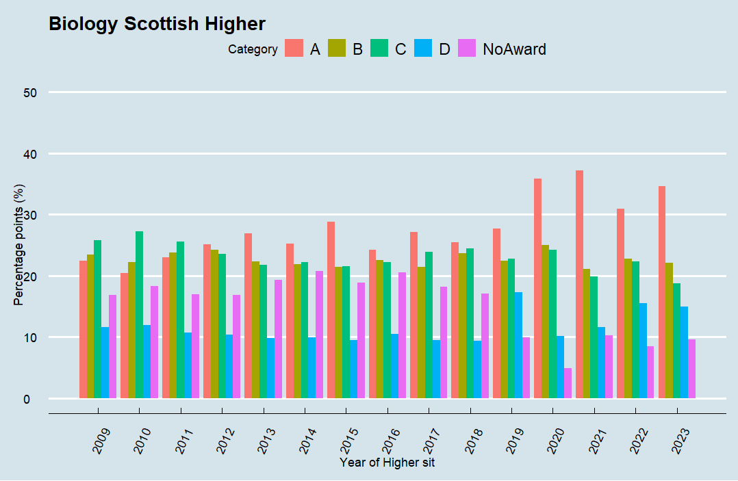
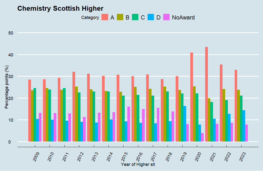
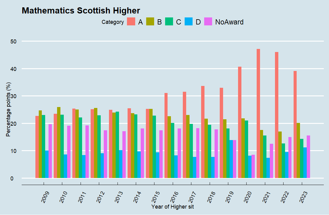
A similar pattern is evident in the four most popular subjects by student entries in 2023.
Biology (7,075 entries)
Chemistry (9,685 entries)
Maths (18,705 entries)
English (35,520 entries)
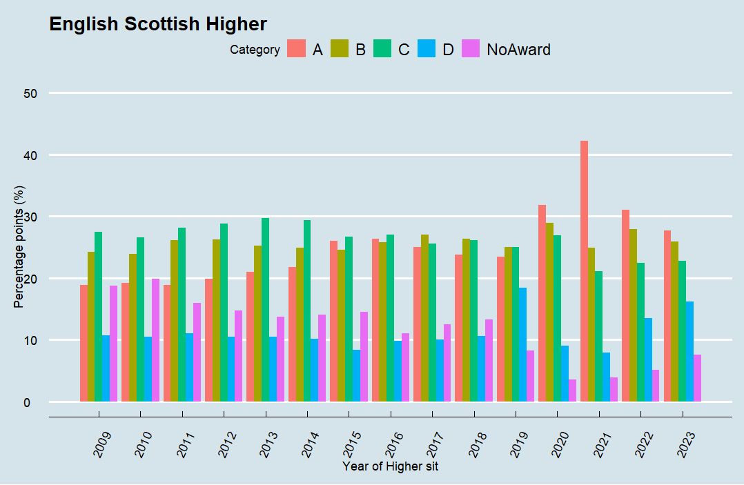
Each subject follows a similar general trend: a gradual increase in top grades before the pandemic, a sharp spike during it, and a subsequent decline — although attainment remains higher than pre-pandemic levels. Part of the surge in top grades can be explained by the shift to teacher-assessed grading, which often produced a more favourable outcome. Improved teaching techniques, better resources and curriculum reform may all have contributed too. Any of these may be a factor, but to state that exams are simply ‘easier’ is harder to prove than the plain fact that Scottish students are attaining better Higher results now than they were ten years ago.
The Impact on University Admissions
A key question remains: What impact does this trend have on university admissions? The following table illustrates what 2023 attainment results would have looked like had they followed the same distribution as in 2009:
| Grade | Expected (2009 distribution) | Actual (2023) | Difference (expected − actual) |
|---|---|---|---|
| A | 48,010 | 63,820 | −15,810 |
| B | 49,495 | 46,025 | 3,470 |
| C | 47,803 | 38,634 | 9,169 |
| D | 16,632 | 25,320 | −8,688 |
| No Award | 29,877 | 18,019 | 11,858 |
Note: The number of total entries was 191,820. These figures represent subject entries rather than individual students; nearly all students sit Higher English, so the number of unique students is closer to 35,520.
In 2023, one-third of students attained an A, up from one-fourth in 2009—an increase that has resulted in over 15,000 additional top grades being awarded. While this does not necessarily suggest students are less capable, it does mean that an A holds less distinguishing value than it did in 2009. This inflation of top grades has forced universities to become more selective, increasing the likelihood that highly qualified school leavers are turned away from institutions such as Glasgow, Edinburgh, and St. Andrews. In response, universities may place greater emphasis on extracurricular achievements — such as volunteering and personal statements — or introduce standardised assessments similar to the SAT in the United States, or the entrance exams used by Oxford and Cambridge. Widening-access policies may also play a growing role: that could mean favouring male candidates, since most universities now admit more women than men (GU 42m:58f, Strath 50m:50f — more the exception than the rule, EdU 38m:62f)*, and it certainly includes the Scottish Government’s target for 20% of higher education entrants to come from the most deprived 20% of the population by 2030.
The sustained rise in top grades within Scottish Highers presents both opportunities and challenges. On the one hand, it may reflect genuine improvements in education, whether through better teaching techniques, enhanced resources, or curriculum reforms. On the other, it raises concerns about grade inflation, particularly its impact on university admissions. If more students achieve top marks, universities must find alternative ways to differentiate applicants — placing greater weight on extracurriculars, personal statements, internal examinations or socio-economic background.
As Scotland moves toward its goal of widening access to higher education, the long-term implications of this trend remain uncertain. Will grade inflation continue, further reshaping university admissions and employer perceptions? Or will standardization efforts stabilize attainment levels? What is clear is that the value of an A today is not what it was in 2009, and institutions—both academic and professional—must adapt accordingly.
* Full-time students during the academic year 2022/23. GU – University of Glasgow; Strath – University of Strathclyde; EdU – University of Edinburgh.
Data source: Fair access to higher education: progress and challenges (Scottish Government), alongside the published SQA attainment spreadsheets.
Code: HerrNiklasLange/SQA_analyses
I will likely write more on the Scottish education system. Ideas on the list:
- grades by sex
- subject preferences by sex
- subject popularity
No guarantees on timing, but I keep coming back to it.
library(dplyr) #library to make programme run
library(sf)
library(leaflet)
library(htmlwidgets)
library(htmltools)
library(formattable)
library(readxl)
library(ggplot2)
library(ggpubr)
library(plyr)
library(tidyr)
library(rstatix)
library(ggplot2)
library(ggthemes)#economist theme

setwd("C:\\Users\\nikla\\programming_projects\\R\\SQL")# change this to the address of the data
##Loading the data for male, female, assement centre & education authority
#This is 2023 to 2019
{
all_H <- read_excel("data/all.xlsx", sheet = 6, range = "A4:BD57")
all_AH <- read_excel("data/all.xlsx", sheet = 7, range = "A4:BD57")
all_nat5 <- read_excel("data/all.xlsx", sheet = 5, range = "A4:BD57")

male_H <- read_excel("data/male.xlsx", sheet = 6, range = "A4:BD57")
male_AH <- read_excel("data/male.xlsx", sheet = 7, range = "A4:BD57")
male_nat5 <- read_excel("data/male.xlsx", sheet = 5, range = "A4:BD57")

female_H <- read_excel("data/female.xlsx", sheet = 6, range = "A4:BD57")
female_AH <- read_excel("data/female.xlsx", sheet = 7, range = "A4:BD57")
female_nat5 <- read_excel("data/female.xlsx", sheet = 5, range = "A4:BD57")

in_H <- read_excel("data/independent.xlsx", sheet = 6, range = "A4:BD57")
in_AH <- read_excel("data/independent.xlsx", sheet = 7, range = "A4:BD57")
in_nat5 <- read_excel("data/independent.xlsx", sheet = 5, range = "A4:BD57")

ot_H <- read_excel("data/other.xlsx", sheet = 6, range = "A4:BD57")
ot_AH <- read_excel("data/other.xlsx", sheet = 7, range = "A4:BD57")
ot_nat5 <- read_excel("data/other.xlsx", sheet = 5, range = "A4:BD57")

co_H <- read_excel("data/college.xlsx", sheet = 6, range = "A4:BD57")
co_AH <- read_excel("data/college.xlsx", sheet = 7, range = "A4:BD57")
co_nat5 <- read_excel("data/college.xlsx", sheet = 5, range = "A4:BD57")


EA_H <- read_excel("data/education-authority.xlsx", sheet = 6, range = "A4:BD57")
EA_AH <- read_excel("data/education-authority.xlsx", sheet = 7, range = "A4:BD57")
EA_nat5 <- read_excel("data/education-authority.xlsx", sheet = 5, range = "A4:BD57")
}
#reading the data of 2018 to 2014 as the way the table is read is different
#test = read_excel("data/pre_2019/2013Higher.xls", sheet = 7, range = "A10:H86")
#test = test
#test2 = read_excel("data/pre_2019/2012Higher.xls", sheet = 8, range = "A10:H86")


reading_pre_2014 <- function(genderBased, N5_H_AH){
  #National 5 did not exists here
  if(genderBased){

  }
  else{ # This is a prime example how inconcinstent government data can be
    #temp0 <- paste("data/pre_2019/2014", N5_H_AH,".xls", sep = "") # Dont need this here
    temp1 = read_excel(paste("data/pre_2019/2013", N5_H_AH,".xls", sep = ""), sheet = 7, range = "A10:H86")
    temp1 = select(temp1, c(-"...6", -"...7"))
    temp1 = fix_grade_pre_2014(temp1, 2013)
    temp2 = read_excel(paste("data/pre_2019/2012", N5_H_AH,".xls", sep = ""), sheet = 8, range = "A10:H85")#Here it is 8
    temp2 = select(temp2, c(-"...6", -"...7"))
    temp2 = fix_grade_pre_2014(temp2, 2012)
    temp3 = read_excel(paste("data/pre_2019/2011", N5_H_AH,".xls", sep = ""), sheet = 8, range = "A10:H83")
    temp3 = select(temp3, c(-"...6", -"...7"))
    temp3 = fix_grade_pre_2014(temp3, 2011)
    temp4 = read_excel(paste("data/pre_2019/2010", N5_H_AH,".xls", sep = ""), sheet = 8, range = "A8:H85") #Need to change
    temp4 = select(temp4, c(-"...6", -"...7"))
    temp4 = fix_grade_pre_2014(temp4, 2010)
    temp5 = read_excel(paste("data/pre_2019/2009", N5_H_AH,".xls", sep = ""), sheet = 7, range = "A6:H81")#Years  Check for AH inconcinstent
    temp5 = select(temp5, c(-"...6", -"...7"))
    temp5 = fix_grade_pre_2014(temp5, 2009)

  }
  df = quickMerge(temp1, quickMerge(temp2, quickMerge(temp3 ,quickMerge(temp4, temp5))))
  return(df %>% drop_na())
}
quickMerge <- function(temp1, temp2){#either N5, Higher or AH
  return(merge(x = temp1, y = temp2, by = "TITLE", all = TRUE))
}
reading_2018_to_2014_grades <- function(genderBased, N5_H_AH){
  if(genderBased){

  }
  else{
    paste("data/pre_2019/2014", N5_H_AH,".xls", sep = "")
    temp1 = read_excel(paste("data/pre_2019/2014", N5_H_AH,".xls", sep = ""), sheet = 6, range = "A8:F73") %>% drop_na()
    temp1 = fix_grade_2014_2018(temp1, "2014")
    temp2 = read_excel(paste("data/pre_2019/2015", N5_H_AH,".xls", sep = ""), sheet = 6, range = "A8:F71")%>% drop_na()
    temp2 = fix_grade_2014_2018(temp2, "2015")
    temp3 = read_excel(paste("data/pre_2019/2016", N5_H_AH,".xls", sep = ""), sheet = 6, range = "A8:F56")%>% drop_na()
    temp3 = fix_grade_2014_2018(temp3, "2016")
    temp3[47,1] = "Total"
    temp4 = read_excel(paste("data/pre_2019/2017", N5_H_AH,".xls", sep = ""), sheet = 6, range = "A8:F56")%>% drop_na()
    temp4 = fix_grade_2014_2018(temp4, "2017")
    temp4[47,1] = "Total"
    temp5 = read_excel(paste("data/pre_2019/2018", N5_H_AH,".xls", sep = ""), sheet = 6, range = "A8:F56")%>% drop_na()
    temp5 = fix_grade_2014_2018(temp5, "2018")
    temp5[47,1] = "Total"
    }
  df = quickMerge(temp1, quickMerge(temp2, quickMerge(temp3 ,quickMerge(temp4, temp5))))
  return(df)
}
fix_grade_pre_2014 <- function(df, year){
  print(year)
  df <- df %>% drop_na()
  df <- df %>% mutate(across(-"TITLE", as.numeric))
  #code to find the the numbers of student who didn't get an award
  df[paste(year,"No Award")] <- round(df[2] - (df[3] + df[4] + df[5] + df[6]), digits = 0)
  return(df)
}
fix_grade_2014_2018 <- function(df, year){
  #df[3] <- as.numeric(df[3])
  #df[4] <- as.numeric(df[4])
  #df[5] <- as.numeric(df[5])
  #df[6] <- as.numeric(df[6])
  df <- df %>% filter(!if_any(everything(), ~ . == "***" | is.na(.)))
  df <- df %>% mutate(across(-"TITLE", as.numeric))
  temp_df <- df
  for (i in 3:(length(df))){

    print((temp_df[i]), n = 50)
    print((temp_df[2]))

    print("Math")
    #print((temp_df[2]/100), n = 50)
    #print(temp_df[i], n = 50)
    #print(round((temp_df[i]) * (temp_df[2])/100), n = 50)
    df[i] = round((temp_df[i]) * ((temp_df[2]))/100)
    print(df[i])

    }
  #code to find the the numbers of student who didn't get an award
  df[paste(year,"No Award")] <- round(df[2] - (df[3] + df[4] + df[5] + df[6]), digits = 0)
  return(df)
}
fix_grade_post_2019 <- function(df){
  #df <- (all_H)
  #This whole thing might result in some rounding errors as the percentages don't make any sense
  new_df <- df["Subject"]
  entries_df <- select(df,contains(c("Entries","Subject")))
  colnames(entries_df)[colnames(entries_df) == 'Entries 2023'] <- '2023 ENTRIES'
  colnames(entries_df)[colnames(entries_df) == 'Entries 2022'] <- '2022 ENTRIES'
  colnames(entries_df)[colnames(entries_df) == 'Entries 2021'] <- '2021 ENTRIES'
  colnames(entries_df)[colnames(entries_df) == 'Entries 2020'] <- '2020 ENTRIES'
  colnames(entries_df)[colnames(entries_df) == 'Entries 2019'] <- '2019 ENTRIES'
  df <- select(df,contains("count"))
  year = 2023
  df[df=="[z]"] <-"0"
  df[df=="[c]"] <-"0"
  for (i in 1:(25)){

    if(grepl("B",colnames(df[i]), fixed=TRUE)){
      print("B")
      print(paste(year,"B"))
      new_df[paste(year,"B")] = strtoi(df[[i]]) - strtoi(df[[i-1]])
    }
    else if(grepl("C Count",colnames(df[i]), fixed=TRUE)){
      print("C")
      print(paste(year,"C"))
      new_df[paste(year,"C")] = strtoi(df[[i]]) - strtoi(df[[i-1]])
    }
    else if(grepl("D",colnames(df[i]), fixed=TRUE)){
      print("D")
      print(paste(year,"D"))

      new_df[paste(year,"D")] = strtoi(df[[i]]) - strtoi(df[[i-1]])
    }
    else if(grepl("No",colnames(df[i]), fixed=TRUE)){
      print("No Award")
      print(paste(year,"No Award"))
      new_df[paste(year,"No Award")] = df[i]


    }
    else{
      print("A")
      print(paste(year,"A"))
      new_df[paste(year,"A")] = df[i]
    }
    if(i %% 5 == 0){
      year = year - 1
    }
  }
  new_df <- merge(new_df, entries_df, by = "Subject")

return(new_df)
}


df1 <- reading_pre_2014(FALSE, "Higher")#No award been given needs to be sorted out
df2 <- reading_2018_to_2014_grades(FALSE, "Higher")
df3 <- fix_grade_post_2019(all_H)

df_all <- merge(x=df3, y=merge(x=df2, y=df1, by.x="TITLE", by.y="TITLE", all = TRUE)[], by.x="Subject", by.y="TITLE", all = TRUE)[]

df_NA <- na.omit(df_all)

rownames(df_NA) <- 1:nrow(df_NA)

df <- df_NA[1:30, ]


#Biology, Chemistry, English, Mathematics, Total

main4 <- df %>% filter(Subject %in% c( "Total", "Biology", "Chemistry", "English", "Mathematics")) #"Biology", "Chemistry", "English", "Mathematics",
{


  df_percentage <- main4%>%
    mutate(across(-"Subject", as.numeric))
  df_percentage <- df_percentage %>%
    mutate(across(-"Subject", as.numeric)) %>%
    mutate(across(starts_with("2023"), ~ round(. / df_percentage$`2023 ENTRIES` * 100, digits = 3)))%>%
    mutate(across(starts_with("2022"), ~ round(. / df_percentage$`2022 ENTRIES` * 100, digits = 3)))%>%
    mutate(across(starts_with("2021"), ~ round(. / df_percentage$`2021 ENTRIES` * 100, digits = 3)))%>%
    mutate(across(starts_with("2020"), ~ round(. / df_percentage$`2020 ENTRIES` * 100, digits = 3)))%>%
    mutate(across(starts_with("2019"), ~ round(. / df_percentage$`2019 ENTRIES` * 100, digits = 3)))%>%
    mutate(across(starts_with("2018"), ~ round(. / df_percentage$`2018 ENTRIES` * 100, digits = 3)))%>%
    mutate(across(starts_with("2017"), ~ round(. / df_percentage$`2017 ENTRIES` * 100, digits = 3)))%>%
    mutate(across(starts_with("2016"), ~ round(. / df_percentage$`2016 ENTRIES` * 100, digits = 3)))%>%
    mutate(across(starts_with("2015"), ~ round(. / df_percentage$`2015 ENTRIES` * 100, digits = 3)))%>%
    mutate(across(starts_with("2014"), ~ round(. / df_percentage$`2014 ENTRIES` * 100, digits = 3)))%>%
    mutate(across(starts_with("2013"), ~ round(. / df_percentage$`2013 ENTRIES` * 100, digits = 3)))%>%
    mutate(across(starts_with("2012"), ~ round(. / df_percentage$`2012 ENTRIES` * 100, digits = 3)))%>%
    mutate(across(starts_with("2011"), ~ round(. / df_percentage$`2011 ENTRIES` * 100, digits = 3)))%>%
    mutate(across(starts_with("2010"), ~ round(. / df_percentage$`2010 ENTRIES` * 100, digits = 3)))%>%
    mutate(across(starts_with("2009"), ~ round(. / df_percentage$`2009 ENTRIES` * 100, digits = 3)))

  df_percentage <- df_percentage %>% select(-contains('ENTRIES'))
  colnames(df_percentage) <- gsub(" ", "", colnames(df_percentage))
  df_percentage[] <- lapply(df_percentage, function(x) if(is.character(x)) x else as.character(x))


  df_graph2 <- df_percentage %>%
    pivot_longer(
      cols = -Subject,
      names_to = c("Year", "Grade"),
      names_sep = "(?<=\\d)(?=[A-Z])",  # Regular expression to separate year and grade
      values_to = "Value"
    )

  # Convert Year to numeric
  df_graph2$Year <- as.numeric(df_graph2$Year)
  df_graph2$Value <- as.numeric(df_graph2$Value)


  {
  ggplot(df_graph2 %>%
           filter(Subject == "Biology"), aes(x = Year, y = Value, fill = Grade)) +
    geom_bar(stat = "identity", position = "dodge") +
    labs(
      #title = "All Scottish Higher results",
      title = "Biology Scottish Higher",
      x = "Year of Higher sit",
      y = "Percentage points (%)",
      fill = "Category"
    ) +
    scale_y_continuous(limits=c(0, 50)) +
    theme_economist() +
    scale_x_continuous(breaks = unique(df_graph2$Year)) +
    theme(axis.text.x = element_text(angle = 65, hjust = 0))
  }#Biology
  {
    ggplot(df_graph2 %>%
             filter(Subject == "Chemistry"), aes(x = Year, y = Value, fill = Grade)) +
      geom_bar(stat = "identity", position = "dodge") +
      labs(
        #title = "All Scottish Higher results",
        title = "Chemistry Scottish Higher",
        x = "Year of Higher sit",
        y = "Percentage points (%)",
        fill = "Category"
      ) +
      scale_y_continuous(limits=c(0, 50)) +
      theme_economist() +
      scale_x_continuous(breaks = unique(df_graph2$Year)) +
      theme(axis.text.x = element_text(angle = 65, hjust = 0))
  }#Chemistry
  {
    ggplot(df_graph2 %>%
             filter(Subject == "English"), aes(x = Year, y = Value, fill = Grade)) +
      geom_bar(stat = "identity", position = "dodge") +
      labs(
        #title = "All Scottish Higher results",
        title = "English Scottish Higher",
        x = "Year of Higher sit",
        y = "Percentage points (%)",
        fill = "Category"
      ) +
      scale_y_continuous(limits=c(0, 50)) +
      theme_economist() +
      scale_x_continuous(breaks = unique(df_graph2$Year)) +
      theme(axis.text.x = element_text(angle = 65, hjust = 0))
  }#English
  {
    ggplot(df_graph2 %>%
             filter(Subject == "Mathematics"), aes(x = Year, y = Value, fill = Grade)) +
      geom_bar(stat = "identity", position = "dodge") +
      labs(
        #title = "All Scottish Higher results",
        title = "Mathematics Scottish Higher",
        x = "Year of Higher sit",
        y = "Percentage points (%)",
        fill = "Category"
      ) +
      scale_y_continuous(limits=c(0, 50)) +
      theme_economist() +
      scale_x_continuous(breaks = unique(df_graph2$Year)) +
      theme(axis.text.x = element_text(angle = 65, hjust = 0))
  }#Mathematics
}